At this moment, we have designed and implemented the Pseudo-Boolean Optimization (PBO) problem set, which contains 25 real-valued test problems on $\{0,1\}^n$. The selection of PBO problems is suggested in Carola Doerr, Furong Ye, Naama Horesh, Hao Wang, Ofer M. Shir, and Thomas Bäck. “Benchmarking discrete optimization heuristics with IOHprofiler.” Applied Soft Computing 88 (2020): 106027.
@article{DoerrYHWSB20,
  author    = {Carola Doerr and
               Furong Ye and
               Naama Horesh and
               Hao Wang and
               Ofer M. Shir and
               Thomas B{\"{a}}ck},
  title     = {Benchmarking discrete optimization heuristics with IOHprofiler},
  journal   = {Appl. Soft Comput.},
  volume    = {88},
  pages     = {106027},
  year      = {2020},
  url       = {https://doi.org/10.1016/j.asoc.2019.106027},
  doi       = {10.1016/j.asoc.2019.106027}
}
Pseudo-Boolean Optimization (PBO) Problem Set
In general, for a pseudo-Boolean function $f\colon \{0,1\}^n \rightarrow \mathbb{R}$, we proposed to creare an instance of it using the following transformation $af(\sigma(x \oplus z)) + b$, in which,
- $z$ is an arbitrary bit string of length $n$ and $\oplus$ denotes the bit-wise XOR function (“translation” in $\{0,1\}^n$),
- $\sigma:[n] \to [n], y \mapsto (y_{\sigma(1)},\ldots,y_{\sigma(n)})$ is a random permutation on the bit string (loosely speaking, “rotation” in $\{0,1\}^n$), and
- $a,b$ are the multiplicative and the additive offset, respectively.
Intuitively, such transformations are devised to test the invariance property of an optimization algorithm, which entails that no performance difference would be measured when the objective function is modified using those transformations. We suggest to apply such transformations on the test functions to challenge your algorithms. Note that, for the continuous optimization problems, this has been practiced in the COCO/BBOB platform, where they applied random affine transformations to test functions.
F1: OneMax
\[\text{OM}:\{0,1\}^n \rightarrow [0..n], x \mapsto \sum_{i=1}^n{x_i}.\]The problem has a very smooth and non-deceptive fitness landscape. Due to the well-known coupon collector effect, it is relatively easy to make progress when the function values are small, and the probability to obtain an improving move decreases considerably with increasing function value.
F2: LeadingOnes
\[\text{LO}:\{0,1\}^n \to [0..n], x\mapsto \max \{i \in [0..n] \mid \forall {j} \le {i}: x_j=1\} = \sum_{i=1}^n{\prod_{j=1}^i{x_j}},\]which counts the number of initial ones.
F3: A Linear Function with Harmonic Weights
\[f:\{0,1\}^n \to \mathbb{R}, x \mapsto \sum_{i} i x_i\]The problem is a linear function with harmonic weights.
F4 - F17: W-model-transformed OneMax and LeadingOnes
The W-model comprises 4 basic transformations, each coming with different instances. We use $W(\cdot,\cdot,\cdot,\cdot)$ to denote the configuration chosen in our benchmark set.
- Dummy variables $W(k,\ast,\ast,\ast)$: this transformation maps each bitstring $(x_1, \ldots, x_n)$ to a substring $(x_{i_1}, \ldots, x_{i_k})$ for the indices $i_1,\ldots, i_k \in [n]$ are randomly chosen and distinct.
- Neutrality $W(\ast,\mu,\ast,\ast)$: The bitstring $(x_1,\ldots,x_n)$ is reduced to a string $(y_1,\ldots,y_m)$ with $m:=\frac{n}{\mu}$, where $\mu$ is a parameter of the transformation. For each $i \in [m]$ the value of $y_i$ is the majority of the bit values in a size-$\mu$ substring of $x$. More precisely, $y_i=1$ if and only if there are at least $\frac{\mu}{2}$ ones in the substring $(x_{(i-1)\mu+1},x_{(i-1)\mu+2},\ldots,x_{i\mu})$. When $\frac{n}{\mu} \notin \mathbb{N}$, the last bits of $x$ are $y$. In our assessment, we regard only the case $\mu=3$.
- Epistasis $W(\ast,\ast,\nu,\ast)$: The idea of epistasis is to introduce local perturbations to the bit strings. To this end, a string $x=(x_1,\ldots,x_n)$ is divided into subsequent blocks of size $\nu$. Using a permutation $e_{\nu}:\{0,1\}^{\nu} \to \{0,1\}^{\nu}$, each substring $(x_{(i-1)\nu+1},\ldots,x_{i\nu})$ is mapped to another string $(y_{(i-1)\nu+1},\ldots,y_{i\nu})=e_{\nu}((x_{(i-1)\nu+1},\ldots,x_{i\nu}))$. The permutation $e_{\nu}$ is chosen in a way that Hamming-1 neighbors $u,v \in \{0,1\}^{\nu}$ are mapped to strings of Hamming distance at least $\nu-1$. In our evaluation, we use $\nu=4$ only.
- Fitness perturbation $W(\ast,\ast,\ast,r)$. With this transformation we can determine the ruggedness and deceptiveness of a function. Unlike the previous transformations, this perturbation operates on the function values, not on the bit strings. To this end, a ruggedness function $r:\{f(x) \mid {x} \in \{0,1\}^n \}=:V \to {V}$ is chosen. The new function value of a string $x$ is then set to $r(f(x))$ , so that effectively the problem to be solved by the algorithm becomes $r \circ f$. We use the following three ruggedness functions.
- $r_1:[0..s] \to [0..\lceil{s/2}\rceil+1$ with $r_1(s)= \lceil {s/2} \rceil +1$ and $r_1(i)=\lfloor {i/2} \rfloor+1$ for $i<s$ and even s, and $r_1(i)=\lceil {i/2} \rceil+1$ for $i<s$ and odd $s$. This function maintains the order of the search points
- $r_2:[0..s] \to [0..s]$ with $r_2(s)=s$, $r_2(i)=i+1$ for $i \equiv s \text{ mod } 2$ and $i<s$, and $r_2(i)=\max{i-1,0}$ otherwise. This function introduces moderate ruggedness at each fitness level.
- $r_3:[0..s] \to [0..s]$ with $r_3(s)=s$ and $r_3(s-5j+k)=s-5j+(4-k)$ for all $j \in {[s/5]}$ and $k {\in} [0..4]$ and $r_3(k)=s - (5\lfloor {s/5} \rfloor - 1 )- k$ for $k \in [0..s - 5\lfloor {s/5} \rfloor -1]$. With this function the problems become quite deceptive, since the distance between two local optima implies a difference of $5$ in the function values.
F4-F17 present superpositions of individual W-model transformations to the OneMax (F1) and the LeadingOnes (F2) problem. Precisely, F4-F17 are
- F4: $\text{OneMax} + W([n/2],1,1,id)$
- F5: $\text{OneMax} + W([0.9n],1,1,id)$
- F6: $\text{OneMax} + W([n],\mu=3,1,id)$
- F7: $\text{OneMax} + W([n],1,\nu=4,id)$
- F8: $\text{OneMax} + W([n],1,1,r_1)$
- F9: $\text{OneMax} + W([n],1,1,r_2)$
- F10: $\text{OneMax} + W([n],1,1,r_3)$
- F11: $\text{LeadingOnes} + W([n/2],1,1,id)$
- F12: $\text{LeadingOnes} + W(0.9n,1,1,id)$
- F13: $\text{LeadingOnes} + W([n],\mu=3,1,id)$
- F14: $\text{LeadingOnes} + W([n],1,\nu=4,id)$
- F15: $\text{LeadingOnes} + W([n],1,1,r_1)$
- F16: $\text{LeadingOnes} + W([n],1,1,r_2)$
- F17: $\text{LeadingOnes} + W([n],1,1,r_3)$
F18: Low Autocorrelation Binary Sequences (LABS)
The Low Autocorrelation Binary Sequences (LABS) problem poses a non-linear objective function over a binary sequence space, with the goal to maximize the reciprocal of the sequence’s autocorrelation:
\[\text{LABS }\colon x\mapsto\frac{n^2}{2\sum_{k=1}^{n-1}\left(\sum_{i=1}^{n-k}s_is_{i+k}\right)^2},\text{ where } s_i=2x_i-1.\]F19-F21: The Ising Model
The classical Ising model considers a set of spins placed on a regular lattice $G=([n],E)$, where each edge $(i,j) \in {E}$ is associated with an interaction strength $J_{ij}$. Given a configuration of $n$ spins, $S:=\left(s_1,\ldots,s_n\right)\in{-1,1}^n$, this problem poses a quadratic function, representing the system’s energy and depending on its structure $J_{ij}$. Assuming zero external magnetic fields and using $x_i = (s_i + 1)/2$ and a unit interaction strength, we obtain the following pseudo-Boolean maximization problem:
\[\text{ISING }\colon x\mapsto \sum\limits_{\\{i,j\\} \in {E}} \left[x_{i}x_{j} + \left(1-x_{i} \right)\left(1-x_{j} \right) \right].\]In PBO, we consider three instances of lattices: the one-dimensional ring (F19), the two-dimensional torus (F20), and the two-dimensional triangular lattice (F21).
F22: Maximum Independent Vertex Set
Given a graph $G=([n],E)$, an independent vertex set is a subset of vertices where no two vertices are are direct neighbors. A maximum independent vertex set (MIVS) is defined as an independent vertex set $V’ \subset [n]$ having largest possible size. Using the standard binary encoding $V’ ={i \in[n] \colon x_i = 1}$, solving MIVS is equivalent to maximizing the following function:
\[\text{MIVS}\colon x\mapsto \sum_i x_i - n\sum_{i,j} x_i x_j e_{ij} = 0.\]F23: N-Queens Problem
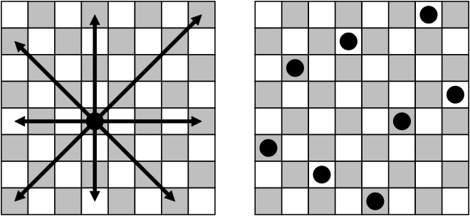
The N-queens problem (NQP) is defined as the task to place N queens on an ${N}\times{N}$ chessboard in such a way that they cannot attack each other. The figure below provides an illustration for the 8-queens problem. Notably, the NQP is actually an instance of the MIVS problem– when consideringa graph on which all possible queen-attacks are defined as edge.
F24: Concatenated Trap
Concatenated Trap (CT) is defined by partitioning a bit-string into segments of length $k$ and concatenating $m=n/k$ trap functions that takes each segment as input. The trap function is defined as follows: $f_k^{\text{trap}}(u) = 1$ if the number $u$ of ones satisfies $u = k$ and $f_k^{\text{trap}}(u) = \frac{k-1-u}{k}$ otherwise. We use $k=5$ in our experiments.
F25: NK landscapes (NKL)
The function values are defined as the average of $n$ sub-functions $F_i \colon [0..2^{k+1}-1] \rightarrow \mathbb{R}, i \in [1..n]$, where each component $F_i$ only takes as input a set of $k \in [0..n-1]$ bits that are specified by a neighborhood matrix. In this paper, $k$ is set to $1$ and entries of the neighbourhood matrix are drawn u.a.r. in $[1..n]$. The function values of $F_i$’s are sampled independently from a uniform distribution on $(0, 1)$.
Links
GitHub Page
Email us
License
BSD 3-Clause
Cite us
Citing IOHprofiler
Developers
Diederick Vermetten
Jacob de Nobel
Furong Ye
Hao Wang
Ofer M. Shir
Carola Doerr
Thomas Bäck