This part is meant for the user who would like a more customizable analysis and visualization experience by manipulating the data directly in an R-environment.
Data structure and manipulation
Here, it is assumed that the data to be loaded follow exactly the aforementioned format regulation. A method DataSetList is provided to load the data:
> dsList <- DataSetList('./data/RLS')
Processing ./data/RLS/IOHprofiler_f1_i1.info ...
   algorithm RLS...
      25 instances on f1 16D...
      25 instances on f1 100D...
...
The return value of method DataSetList is a S3 object, that is inherited from the list class. Consequently, list object can be sliced, indexed and printed as with lists:
> dsList
DataSetList:
1: DataSet(RLS on f1 16D)
2: DataSet(RLS on f1 100D)
---
7: DataSet(RLS on f23 16D)
8: DataSet(RLS on f23 100D)

> dsList[1:3]
DataSetList:
1: DataSet(RLS on f1 16D)
2: DataSet(RLS on f1 100D)
3: DataSet(RLS on f19 16D)

> dsList[[1]]
DataSet(RLS on f1 16D)
In addition, the summary method is implemented to show some basic information:
> summary(dsList)
  funcId DIM algId                                           datafile comment
1      1  16   RLS     ./data/RLS/data_f1/IOHprofiler_f1_DIM16_i1.dat       %
2      1 100   RLS    ./data/RLS/data_f1/IOHprofiler_f1_DIM100_i1.dat       %
3     19  16   RLS   ./data/RLS/data_f19/IOHprofiler_f19_DIM16_i1.dat       %
4     19 100   RLS  ./data/RLS/data_f19/IOHprofiler_f19_DIM100_i1.dat       %
5      2  16   RLS     ./data/RLS/data_f2/IOHprofiler_f2_DIM16_i1.dat       %
6      2 100   RLS    ./data/RLS/data_f2/IOHprofiler_f2_DIM100_i1.dat       %
7     23  16   RLS   ./data/RLS/data_f23/IOHprofiler_f23_DIM16_i1.dat       %
8     23 100   RLS  ./data/RLS/data_f23/IOHprofiler_f23_DIM100_i1.dat       %
Note that, column funcId stands for the numbering (ID) of test functions and algId is the identifier of the algorithm that is tested. Those columns (also DIM) are the attribute of list object, which are directly retrieved from the meta data (*.info files). Therefore, it is important to keep the meta data correct if it were prepared by the user manually. All the attributes DataSetList object are listed as follows:
> attributes(dsList)
$class
[1] "list"        "DataSetList"

$DIM
[1]  16 100  16 100  16 100  16 100

$funcId
[1]  1  1 19 19  2  2 23 23

$algId
[1] "RLS" "RLS" "RLS" "RLS" "RLS" "RLS" "RLS" "RLS"
When subsetting (filtering) is needed for list, attributes DIM, funcId and algId can be used as follows:
> subset(dsList, DIM == 16, funcId == 1)
DataSetList:
1: DataSet(RLS on f1 16D)

> subset(dsList, DIM == 16, algId != 'RLS')
DataSetList:
Now we could load the data files of the $(1,\lambda)$-GA algorithm in the same way:
> dsList_ga <- DataSetList('./data/self_GA', verbose = FALSE)
Here, the argument verbose is set to FALSE to hide the prompting message. As with the R list, DataSetList objects can be combined together:
> dsList <- c(dsList, dsList_ga)
Each element of list is a S3 object of type DataSet, which is again inherited from the list class.
> ds <- dsList[[1]]
> ds
DataSet(RLS on f1 16D)

> summary(ds)
DataSet Object:
Algorithm: RLS
Function ID: 1
Dimension: 16D
25 instance found: 1,1,1,1,1,2,2,...,4,4,4,5,5,5,5,5

runtime summary:
    algId target  mean median        sd 2% 5% 10% 25% 50% 75% 90% 95% 98%   ERT runs ps
 1:   RLS      4  1.00      1  0.000000  1  1   1   1   1   1   1   1   1  1.00   25  1
 2:   RLS      5  1.04      1  0.200000  1  1   1   1   1   1   1   1   1  1.04   25  1
 3:   RLS      6  1.28      1  1.208305  1  1   1   1   1   1   1   2   2  1.28   25  1
 ---
11:   RLS     14 21.00     21  9.165151  5  5   7  14  18  26  34  37  37 21.00   25  1
12:   RLS     15 29.16     29 10.466932 12 12  15  18  26  36  40  48  48 29.16   25  1
13:   RLS     16 46.48     48 21.652790 13 13  19  26  42  58  71  83  83 46.48   25  1

function value summary:
    algId runtime runs  mean median        sd    2%   5%  10% 25% 50% 75%  90%  95%   98%
 1:   RLS       1   25  7.68      7 1.7729448  4.48  5.2  6.0   7   7   9 10.0 10.8 11.00
 2:   RLS       2   25  8.28      8 1.6206994  5.48  6.0  6.4   7   8   9 10.0 10.8 11.52
 3:   RLS       3   25  8.76      9 1.5885003  5.48  6.2  7.0   8   9  10 10.6 11.0 11.52
---
64:   RLS    2511   25 16.00     16 0.0000000 16.00 16.0 16.0  16  16  16 16.0 16.0 16.00
65:   RLS    2818   25 16.00     16 0.0000000 16.00 16.0 16.0  16  16  16 16.0 16.0 16.00
66:   RLS    3162   25 16.00     16 0.0000000 16.00 16.0 16.0  16  16  16 16.0 16.0 16.00

Attributes: names, class, suite, funcId, DIM, algId, algInfo, comment, datafile, instance,
  maxRT, finalFV, format, maximization
In the summary method, the data set is summarized in two perspectives:
- Fixed-target perspective: the method looks for the first hitting time, that is the number of function evaluations an algorithm takes to reach a target function value (target above) for the first time. The target values are automatically determined and evenly spaced in the observed range. Some basic statistics on the running time sample are calculated for each target value: mean, median, standard deviation (sd), percentiles (2% 5% 10% …), the expected running time (ERT) and success rate (ps, the ratio of successful runs our of all the independent runs).
- Fixed-budget perspective: the method looks for the best function value reached by the algorithm, when a specific number of function evaluations (budget) are taken (runtime above). The budget values are automatically determined and evenly spaced in the observed range. Roughly the same set of statistics are provided as the fixed-target perspective.
In the ds object, two matrices are always stored for those two perspectives explained above:
ds$RT: running time samples in the fixed-target perspective andds$FV: function value samples in the fixed-budget perspective.
Note that, when the parameter tracking is enabled, the parameter of interest is also arranged in the fixed-target perspective and is appended to ds object. For instance, if mutation_rate is the parameter name given to the benchmark, the parameter can be obtained by ds$mutation_rate. We could take a glimpse at those two matrices:
> head(ds$RT)
   [,1] [,2] [,3] [,4] [,5] [,6] [,7] [,8] [,9] [,10] [,11] [,12] [,13] [,14]
4    1    1    1    1    1    1    1    1    1     1     1     1     1     1
5    1    1    1    1    1    1    1    1    1     1     1     2     1     1
6    1    1    1    1    1    1    1    1    2     1     1     7     1     1
7    1    1    1    1    1    3    1    1    5     1     1     8     1     1
8    1    3    2    2    1    4    1    1    7     2     1    10     2     1
9    1    4    3    3    4    5    1    1    8     4     2    11     3     1
Here, the column names are the target values and in the example below, those are the budget values:
> head(ds$FV)
   [,1] [,2] [,3] [,4] [,5] [,6] [,7] [,8] [,9] [,10] [,11] [,12] [,13] [,14]
1   11    7    7    7    8    6    9    9    5     7     8     4     7    11
2   11    7    8    8    8    6    9   10    6     8     9     5     8    12
3   11    8    9    9    8    7   10   10    6     8     9     5     9    12
4   12    9   10    9    9    8   10   11    6     9    10     5     9    13
5   12    9   10    9   10    9   10   12    7    10    10     5    10    14
6   13    9   11   10   10   10   10   13    7    11    11     5    10    14
Retrieving performance data
For both DataSet and DataSetList objects, the overview of the observed running time/function value can obtained using:
> get_RT_overview(subset(dsList, algId == 'RLS'))
   Algorithm DIM fID miminal runtime maximal runtime runs Budget
1:       RLS  16   1               1              96   25  16000
2:       RLS 100   1               1            1128   25 100000
3:       RLS  16  19               1              52   25  16000
4:       RLS 100  19               1             570   25 100000
5:       RLS  16   2               1             255   25  16000
6:       RLS 100   2               1            6546   25 100000
7:       RLS  16  23               1              67   25  16000
8:       RLS 100  23               1             641   25 100000

> get_RT_overview(ds)
   algId DIM funcId miminal runtime maximal runtime runs Budget
1:   RLS  16      1               1              96   25  16000
Here, Budget indicates the maximal allowable budget that is given when running the experiment while maximal runtime is the maximal observed running time in each triplet of (algId, DIM, funcId). For the function values, the similar methods are also implemented:
> get_FV_overview(subset(dsList, algId == 'RLS'))
   algId DIM funcId worst recorded worst reached best reached mean reached median reached runs succ budget
1:   RLS  16      1              4            16           16        16.00             16   25   25  16000
2:   RLS 100      1             44           100          100       100.00            100   25   25 100000
3:   RLS  16     19              8            20           32        25.60             24   25    1  16000
4:   RLS 100     19             92           152          172       162.56            164   25    3 100000
5:   RLS  16      2              0            16           16        16.00             16   25   25  16000
6:   RLS 100      2              0           100          100       100.00            100   25   25 100000
7:   RLS  16     23           -100             3            4         3.24              3   25    6  16000
8:   RLS 100     23          -1868             7            9         8.20              8   25    9 100000
It is important to distinguish some columns in the example here: worst recorded stands for the worst (smallest) function value observed in all independent runs for each case of (algId, DIM, funcId). In contrast, worst reached means the smallest value reached in the last iteration (across independent runs) of the algorithm while best reached the largest value. runs gives the total number of independent runs in each case while succ is the number of runs where the corresponding best reached is hit. Note that, in our naming convention of methods, RT is always the abbreviation of running time and FV is for function value (the same below). To get a data summary at arbitrary running time/function value, two methods, get_RT_summary and get_FV_summary are implemented. Let use the object ds (defined before) to illustrate the usage:
> ds
DataSet(RLS on f1 16D)
> get_RT_summary(ds, ftarget = c(5, 10, 16))
   algId target  mean median        sd 2% 5% 10% 25% 50% 75% 90% 95% 98%   ERT runs ps
1:   RLS      5  1.04      1  0.200000  1  1   1   1   1   1   1   1   1  1.04   25  1
2:   RLS     10  5.24      5  3.455431  1  1   1   2   5   6  10  12  12  5.24   25  1
3:   RLS     16 46.48     48 21.652790 13 13  19  26  42  58  71  83  83 46.48   25  1

> get_FV_summary(ds, runtime = c(10, 50, 100))
   algId runtime runs  mean median        sd    2% 5%  10% 25% 50% 75% 90%  95% 98%
1:   RLS      10   25 11.52     12 1.5307950  8.48  9  9.4  11  12  13  13 13.8  14
2:   RLS      50   25 15.64     16 0.4898979 15.00 15 15.0  15  16  16  16 16.0  16
3:   RLS     100   25 16.00     16 0.0000000 16.00 16 16.0  16  16  16  16 16.0  16
The input for the argument ftarget and runtime should be provided by the user. In this example, three values are chosen arbitrarily in the corresponding range of running time/function value (cf. the first lines of get_RT_overview and get_FV_overview above). Furthermore, using the magrittr package (please install it if necessary), it is possible to chain all the methods introduced so far, making the code snippet more readable:
> library(magrittr)
> dsList %>%
+   subset(DIM == 100, algId == 'RLS', funcId == 19) %>%
+   get_FV_summary(runtime = seq(1, 5000, length.out = 5))
   DIM funcId algId runtime runs   mean median       sd  2%    5%   10% 25% 50% 75%   90% 95% 98%
1: 100     19   RLS    1.00   25 104.16    104 8.284926  92  92.0  93.6 100 104 108 116.8 120 120
2: 100     19   RLS 1250.75   25 162.56    164 6.096994 152 152.8 156.0 156 164 168 170.4 172 172
3: 100     19   RLS 2500.50   25 162.56    164 6.096994 152 152.8 156.0 156 164 168 170.4 172 172
4: 100     19   RLS 3750.25   25 162.56    164 6.096994 152 152.8 156.0 156 164 168 170.4 172 172
5: 100     19   RLS 5000.00   25 162.56    164 6.096994 152 152.8 156.0 156 164 168 170.4 172 172
In addition, it is also straightforward to retrieve the raw sample points of the running time/function value, using the following methods, get_RT_sample and get_FV_sample:
> get_RT_sample(ds, ftarget = 10, output = 'long')
    algId target run RT
 1:   RLS     10   1  1
 2:   RLS     10   2  8
 3:   RLS     10   3  4
---
23:   RLS     10  23 12
24:   RLS     10  24  1
25:   RLS     10  25  8
> get_FV_sample(ds, runtime = c(5, 20), output = 'wide')
   algId runtime run.1 run.2 run.3 run.4 run.5 run.6 run.7 run.8 run.9 run.10 run.11 run.12
1:   RLS       5    12     9    10     9    10     9    10    12     7     10     10      5
2:   RLS      20    16    12    15    14    14    13    14    15    14     12     14     13
Note that, all methods in this sub-section return a data.table object from the data.table package.
Plotting
To visualize the benchmark data, a collection of plotting methods are implemented in \iohana. In this section, we shall provide examples on some important plots using the data set in the last section. Here, only the plotting method for the fixed-target perspective is shown because the same set of methods are implemented for the fixed-budget perspective. Firstly, the progression of the function value is plotted against the running time:
> ds_plot <- subset(dsList, DIM == 16, funcId == 1)
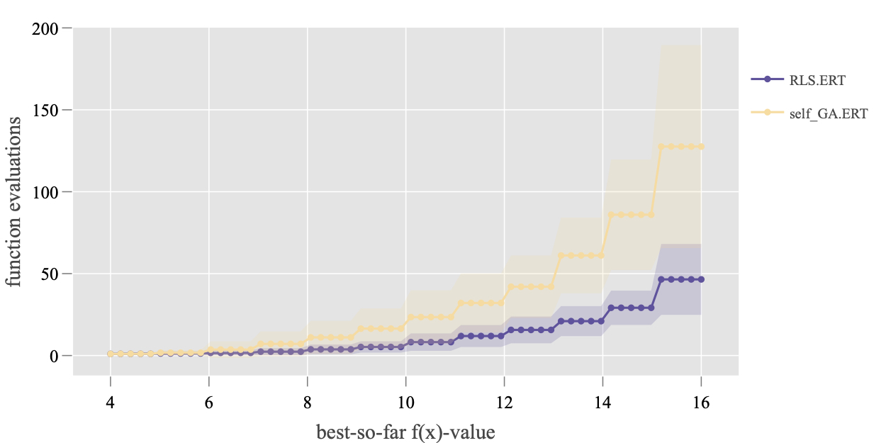
> Plot.RT.Single_Func(ds_plot)
The data sets on 16D, function F1 are plotted here, which is shown in the following figure. Note that, a interactive plot is created as the plotly library is used here by default. The static plotting library ggplot2 can also be selected by setting argument backend = 'ggplot2' (this is only a difference in the plotting backend and thus it will not be demonstrated here). In the figure, the standard deviation of the running time is also drawn.
> ?Plot.RT.Single_Func
In addition, the previous plot can be grouped by functions, using Plot.RT.Multi_Func methods. The example is shown below.
> Plot.RT.Multi_Func(ds_plot, scale.ylog = T)

Given a target value, Plot.RT.Histogram methods renders the histogram of the running time required to reach this target value. Taking the data set on F23 and 16D as an example, it is important to view the range of function values through method get_FV_overview as shown in the previous section:
> ds <- subset(dsList, DIM == 16, funcId == 23)
> get_FV_overview(ds)
       algId DIM funcId worst recorded worst reached best reached ... Budget
1:       RLS  16     23           -100             3            4 ...  16000
2:   self_GA  16     23            -96             4            4 ...  16001
Then, we choose a target value -3 that is close to the best reached value and plot the histogram.
> Plot.RT.Histogram(ds, ftarget = -3, plot_mode = 'subplot')
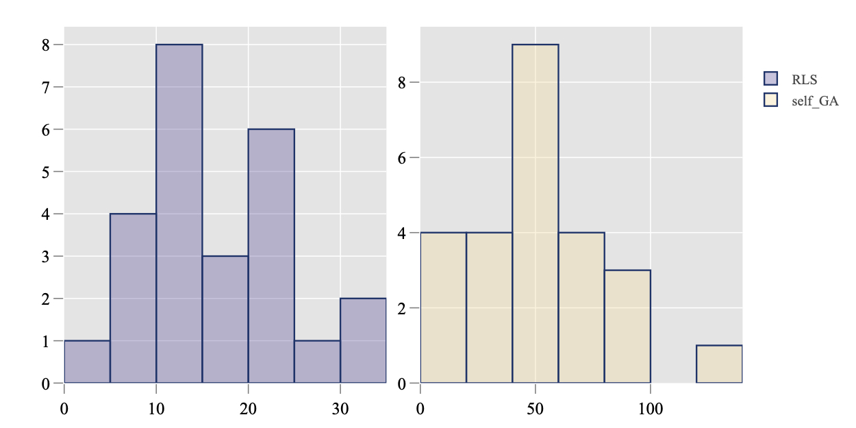
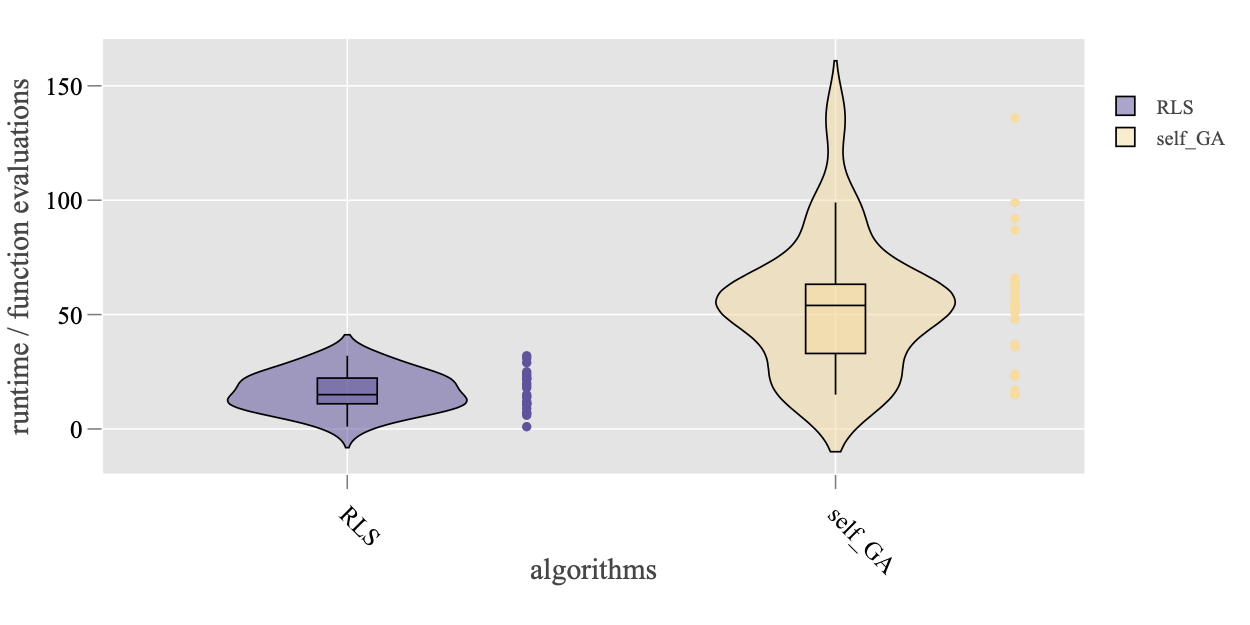
The argument plot_mode = 'subplot' will create a separate sub-plot for each algorithm in the data set. In addition, the empirical density function of the running time, that is estimated by the Kernel Density Estimation (KDE) method, can be generated by method Plot.RT.PMF.
> Plot.RT.PMF(ds, ftarget = -3, show.sample = TRUE)
Finally, it is also crucial to look at the Empirical Cumulative Distribution function (ECDF) of the running time. For this purpose, three methods are implemented for different levels of data aggregation:
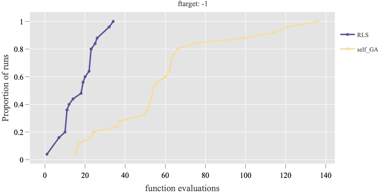
Plot.RT.ECDF_Per_Target: it only compares the ECDF of algorithms on a single target value, e.g.,
> Plot.RT.ECDF_Per_Target(ds, ftarget = -1)
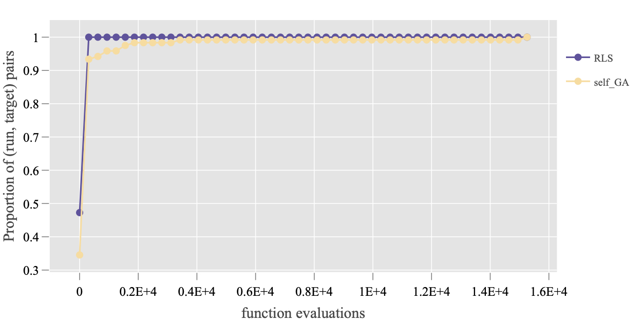
Plot.RT.ECDF_Single_Func: it takes as input an array of target values (controlled by arguments fstart, fstop, fstep) and aggregates the ECDF over those targets, e.g.,
> Plot.RT.ECDF_Single_Func(ds, fstart = -92, fstop = 4, fstep = 10)
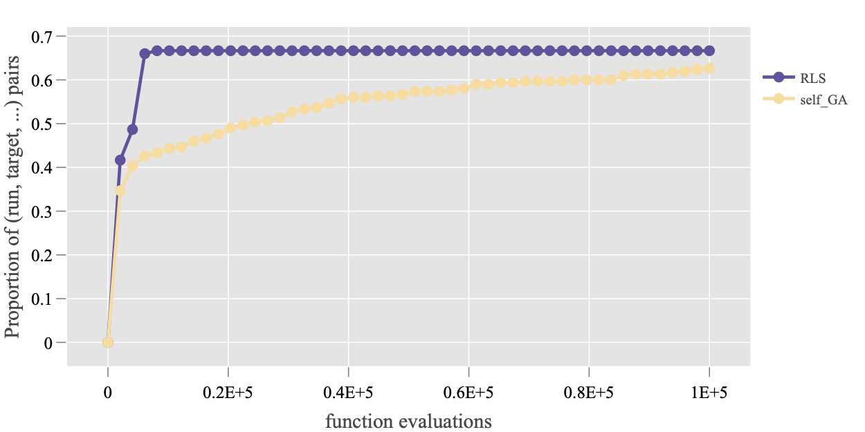
Plot.RT.ECDF_Multi_Func: This ECDF plot also aggregates different target values over all test function in the data set. To demonstrate its usage, let’s take the data set on 100D and check the overview of the function values. Then three target values are chosen manually for each function, which are collected in a list object. The resulting plot is shown in the figure below.
> ds <- subset(dsList, DIM == 100)
> get_FV_overview(ds)
     algId DIM funcId worst recorded worst reached best reached ... budget
1:     RLS 100      1             44           100          100 ... 100000
2:     RLS 100     19             92           152          172 ... 100000
3:     RLS 100      2              0           100          100 ... 100000
4:     RLS 100     23          -1868             7            9 ... 100000
5: self_GA 100      1             38            98          100 ... 100001
6: self_GA 100     19             72           164          192 ... 100001
7: self_GA 100      2              0            39          100 ... 100001
8: self_GA 100     23          -1761             7           10 ... 100001

> ftarget <- list(`1` = c(80, 90, 100),
+                  `2` = c(80, 90, 100),
+                  `19` = c(180, 190, 200),
+                  `23` = c(0, 5, 10))

> Plot.RT.ECDF_Multi_Func(ds, ftarget)
Links
GitHub Page
Email us
License
BSD 3-Clause
Cite us
Citing IOHprofiler
Developers
Diederick Vermetten
Jacob de Nobel
Furong Ye
Hao Wang
Ofer M. Shir
Carola Doerr
Thomas Bäck