To guide you through the GUI of IOHanalyzer, please feel free to use either

• The free GUI server hosted at http://iohprofiler.liacs.nl/, or
• Starting up the GUI locally given IOHanalyzer is already installed:

> runServer()
Loading required package: shiny

Listening on http://127.0.0.1:xxxx

This command will start the GUI server on your local machine (using the IP address 127.0.0.1 and a random port number). The web browser will be launched and connect to this address immediately after starting the server. The functionalities are grouped as follows:

• Upload Data: This section provides functionality to upload experiment results or load an official data set that is provided by the author.
• Fixed-Target Results This section provides statistics covering the fixed-target perspective of performance evaluation. That is, the results in this section mainly address the question about the statistical property of running time (i.e., function evaluations) that is needed to obtain a solution of a desired target quality.
• Fixed-Budget Results This section covers the fixed-budget perspective, that is the statistics on objective function values obtained by the search points a given budget of function evaluations. In other words, the results in this section mainly address the question how good the search points are that a user can expect to see within a given frame of running time.

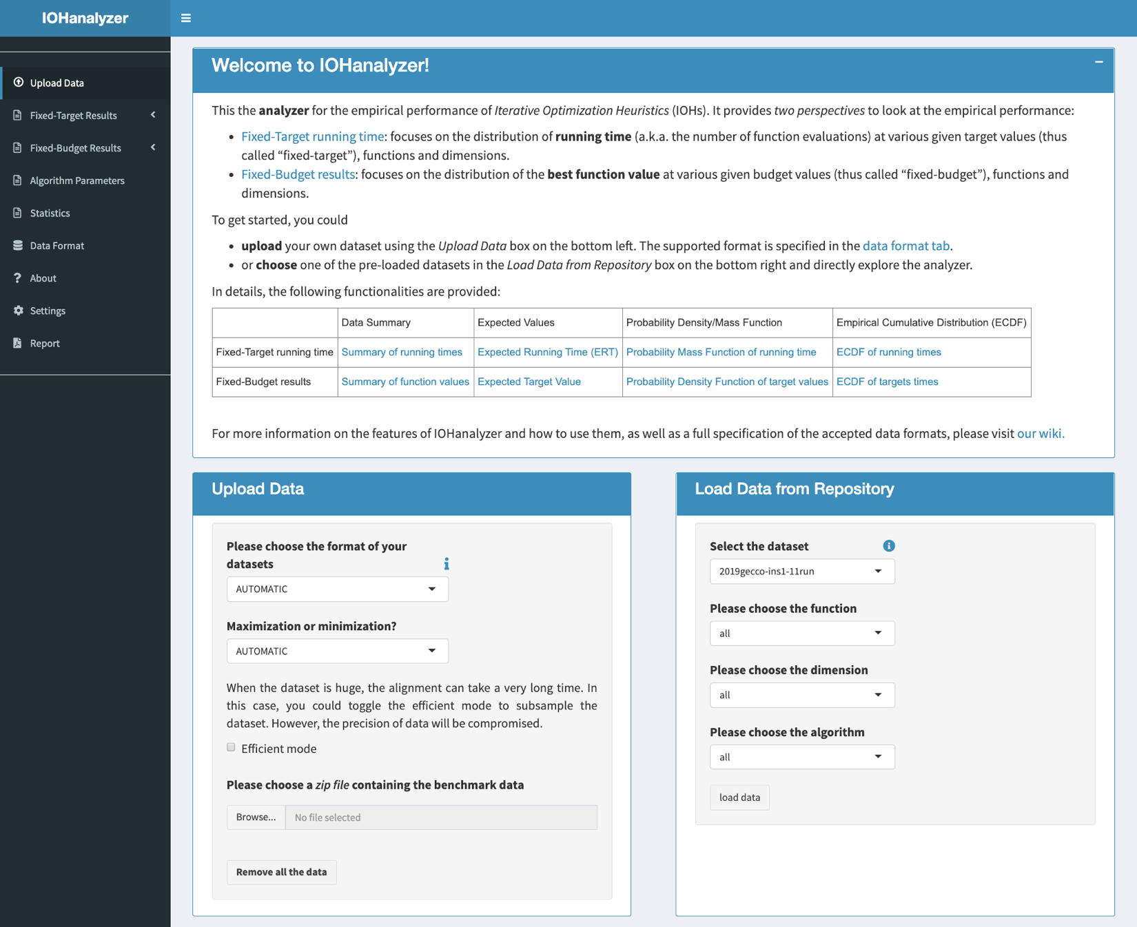
Upload data

The GUI interface to load the experiment data is shown in the following figure, in which the user is asked to upload a compressed archive. The following compression format are supported: *.zip, *.bz, *.tar, *.xz, *.gz. Note that, when the user’s data set is enormous to handle, it is possible to speed up the uploading (and hence plotting) procedure by toggling option Efficient mode on, in which a subset is taken from the huge data set. Moreover, when using the online GUI, the user can also load official data sets provided by the author, using the Load Data from Repository box on the right of the page. At the time of writing, two official data sets are made available, each of which contains results of 11 algorithms on all 23 test functions, over dimensions {16, 100, 625}. For the specification of those two data sets and updates on the data set, the user is suggested to visit data page.

Fixed-target results

The fixed-target section has four different subsections:

• Data Summary
• Expected Runtime
• Probability Mass Function
• Cumulative Distribution

Data Summary

It provides some statistics on the running time $T(A, f, d, v)$, meaning the function evaluation an algorithm $A$ would require to reach target value $v$ of test function $f$ on dimension $d$. In the following, the indexing parameter in $T$ will be dropped if no ambiguity is created. Assuming a number of independent runs of algorithm $A$ is performed on the tuple of $(f, d, v)$, the set of results from all runs $(t_i)_i$ is considered as a simple random sample of $T$. Here, three tables are provided to summarize the sample $(t_i)_i$ of $T$:

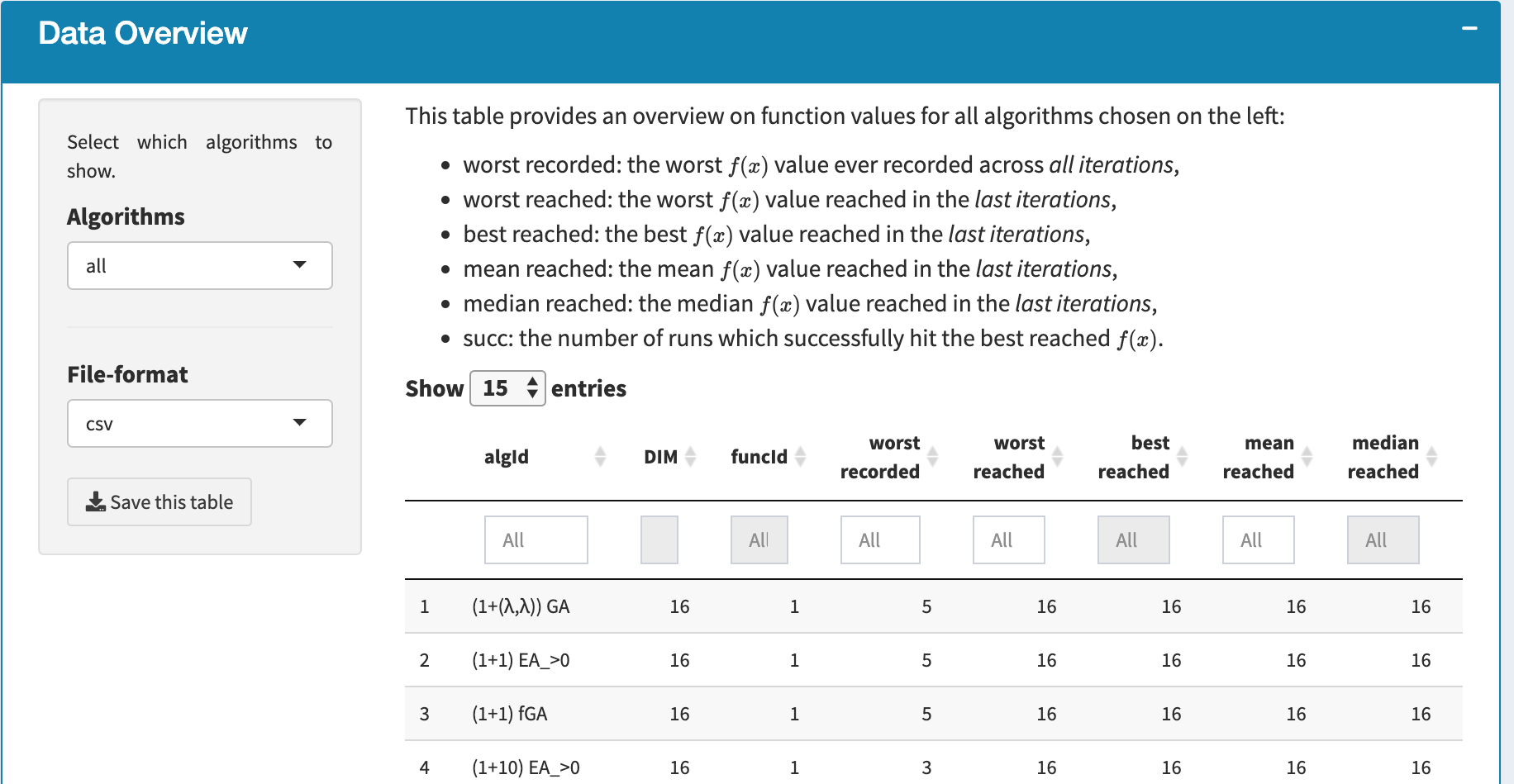
• Data Overview A screenshot of this table is given as below. As counterintuitive as it may seem, this table contains the overview of the function value observed in a data set. The main reason of showing this table here is to provide the user a quick summary of the range of function value, which is required to play with the following two functionalities.

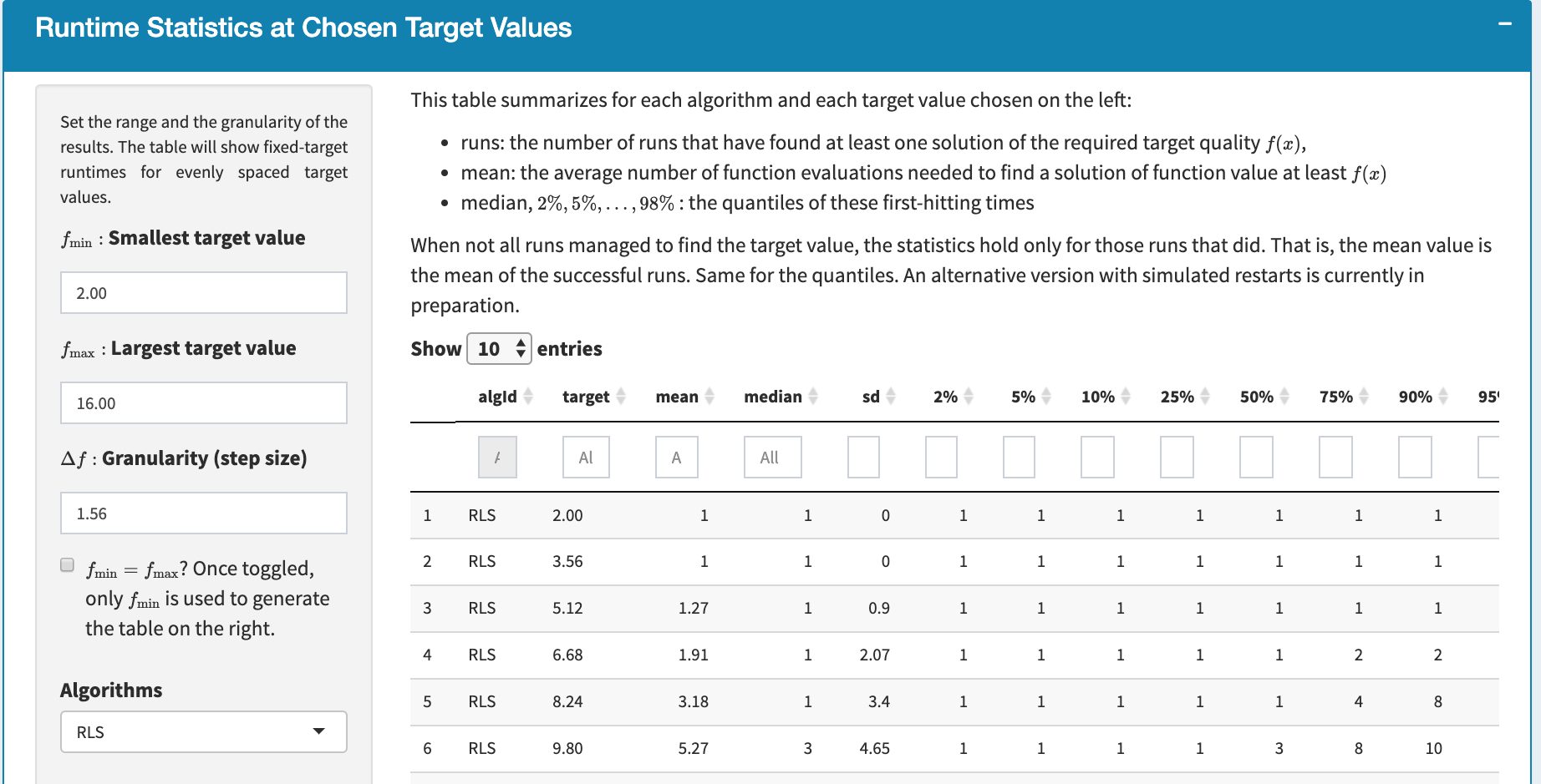
• Runtime Statistics at Chosen Target Values A screenshot of this table is given as below. The table is obtained from The user can set the range and the granularity of the results in the box on the left. The table shows fixed-target running times for evenly spaced target values. More precisely, for each tuple of (algorithm $A$, target value $v$, dimension $d$) the table provides 1) successful runs: the number of runs (sample points) of algorithm $A$ in which at least one solution $x$ satisfying $f(x)>v$ has been found 2) sample mean, median, standard deviation 3) sample quantiles: $Q_{2\%}, Q_{5\%},\ldots, Q_{98\%}$ and 4) the expected running time (ERT). Additionally, the user can also download this table in CSV format, or as a LaTeX table.

• Original Runtime Samples The user interface is similar to the previous except that the sample points $(t_i)_{i}$ of running time $T(A, f, d, v)$ is shown here. Moreover, the user can choose between a long (all sample points are stored in a column) and a wide format (all sample points are stored in a row) for the table.

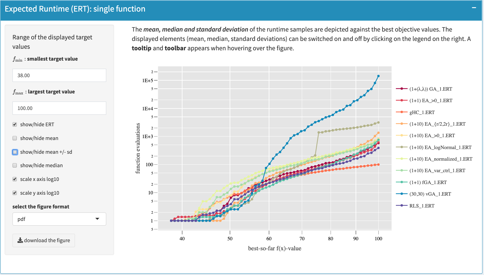
Expected runtime

An interactive plot (using shiny package) illustrates the fixed-target running times. An example of this plot is shown as below as below. The interactive plot can be adjusted by a couple of options on the left menu as shown in figure, including showing/hiding mean and/or median values along with standard deviations and scaling axis logarithmically. The user also selects the algorithms to be displayed, the range of target values within which the curves are drawn. The displayed curves can be switched on and off by clicking on the legend on the right of the plot. In addition, the figure can be downloaded in the following format: pdf, eps, svg and png (which also applies to all the plots hereafter).

Probability mass function

For a selected target value $v$, the histogram of the running time, as displayed below,

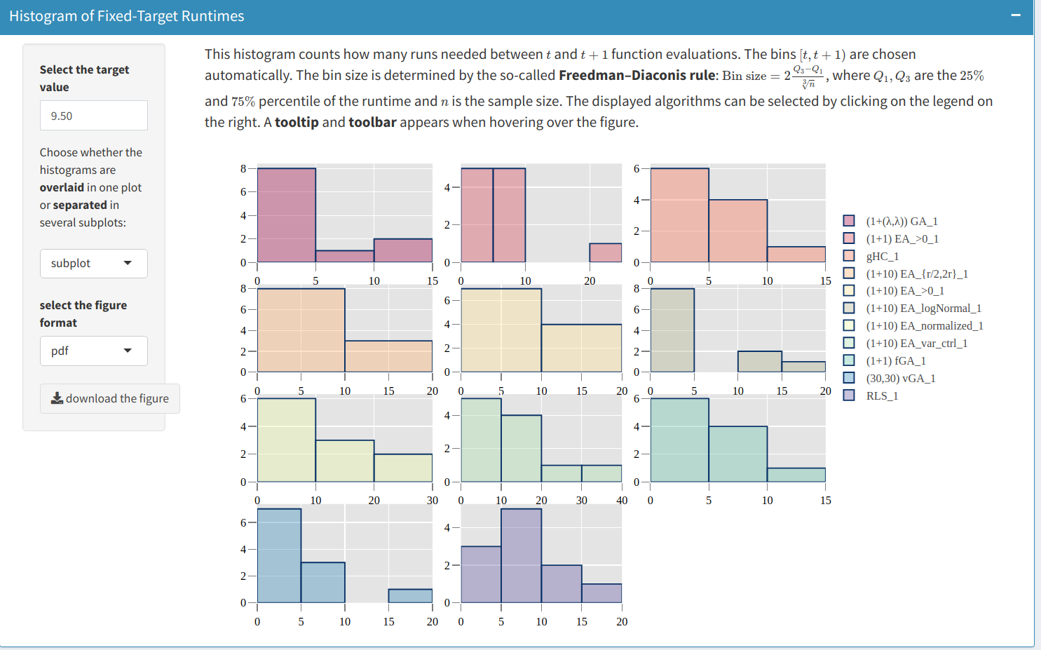
shows the number of runs $i$ where the running time falls into a given interval $[t,t+1)$, namely $t \le t_i(A,f,d,v) < t+1$. The bin size $[t,t+1)$ is automatically determined according to the so-called Freedman-Diaconis rule, which is based on the interquartile range of sample $(t_i)_i$. The user has two options:

• Overlayed display, where all algorithms are displayed in the same plot
• Separated one, where each algorithm is displayed in an individual sub-plot.

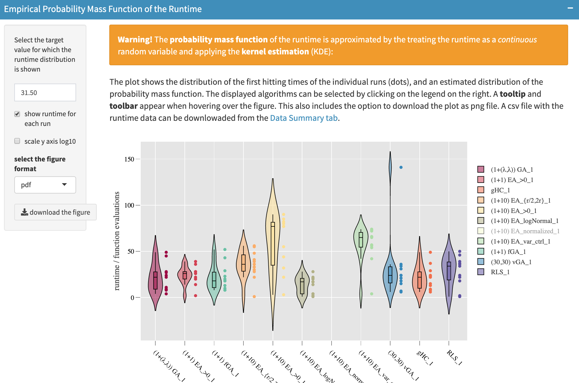
In addition to the histogram, the empirical probability mass function (see figure below) might be helpful to get a finer look at the shape of the empirical distribution of $T(A,f,d,v)$. The user can opt to show all sample points $(t_i)_{i}$ for each algorithm (which will be plotted as dots), or only the empirical probability mass function itself. It is important to point out that the probability mass function is estimated in a “continuous” manner, where running time samples are considered as $\mathbb{R}$-valued and then a Kernel Density Estimation (KDE) is taken to obtain the curve. Note also that in the figure many sample points seem overlapping, this might be caused by turning (in the data upload part) the efficient mode on, in which the raw data set is trimmed.

Cumulative distribution

The empirical cumulative distribution function of the running time are computed for target values specified by the user. In addition to showing ECDFs for a single target value, it is recommended to aggregate ECDFs over multiple target, to obtain an overall performance profile for all algorithms. This functionality is exemplified below:

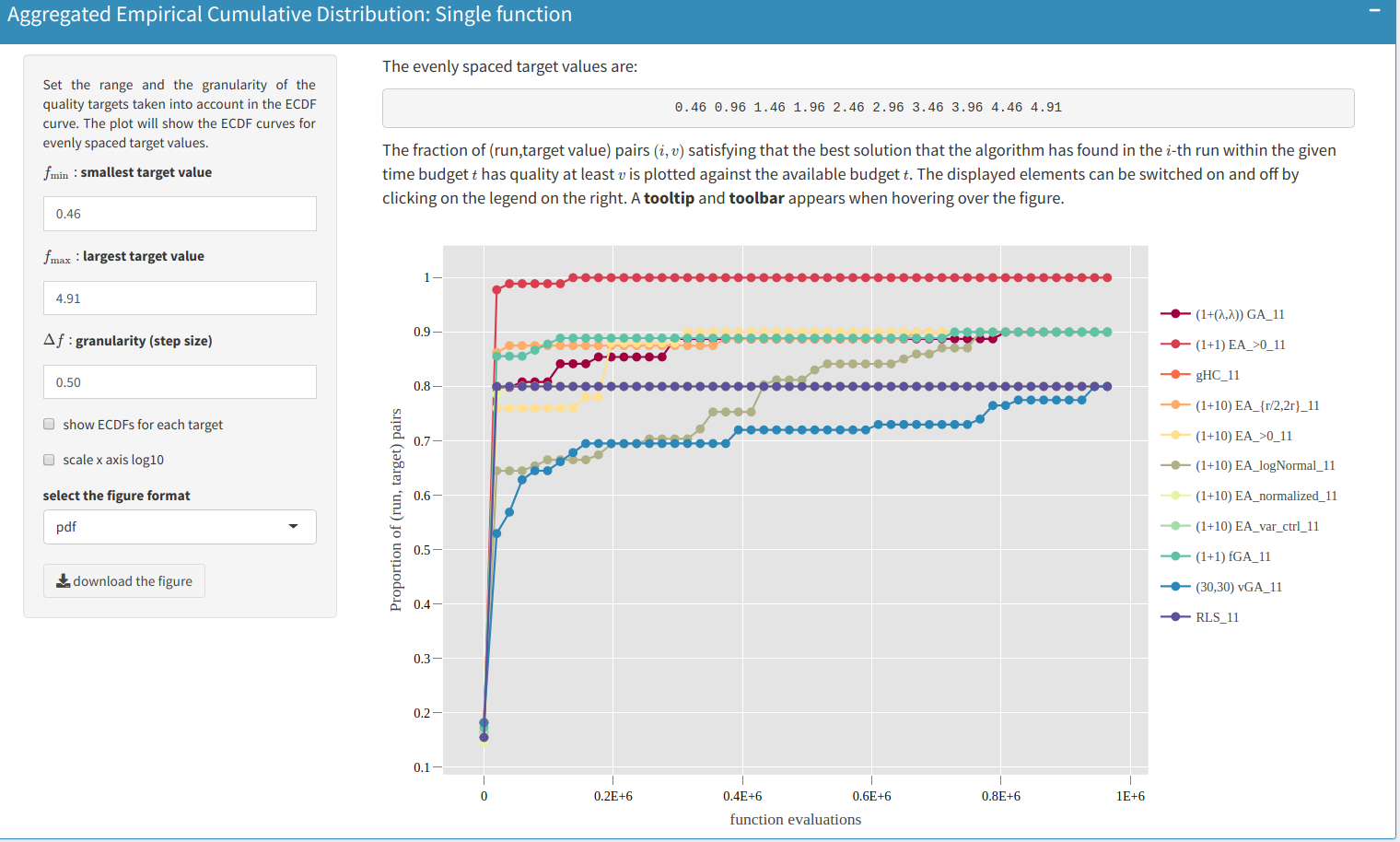
A set of evenly spaced target value can be generated by specifying the range and step of the target value. In this example, with the following setup, $f_{\min}=0.46$, $f_{\max}=4.91$, and $\Delta f=0.5$, the ECDF curves for target values $0.46,0.96,1.46,\ldots, 4.91$ are computed. The aggregation across targets is defined in the following sense: for a set of target values $V$, $r$ number of independent runs on each function, the aggregated ECDF considers running time samples of all target values and runs together. In the upper figure, for algorithm $(30,30)$-vGA (blue curve) this is the case for around $70\%$ of the pairs after $t=2\,0000$ function evaluations. For algorithm RLS (purple curve) the fraction is $80\%$.

Ideally, the best algorithm would sample the maximal function value $f_{\max}$ in the first function evaluation. This algorithm would have a $100\%$ cumulative probability for any running time. In practice, such an algorithm does not exist, but it serves as a theoretical upper bound. Furthermore, this way of performing the aggregation can be leveraged to a set of test functions, as shown in the following plot:

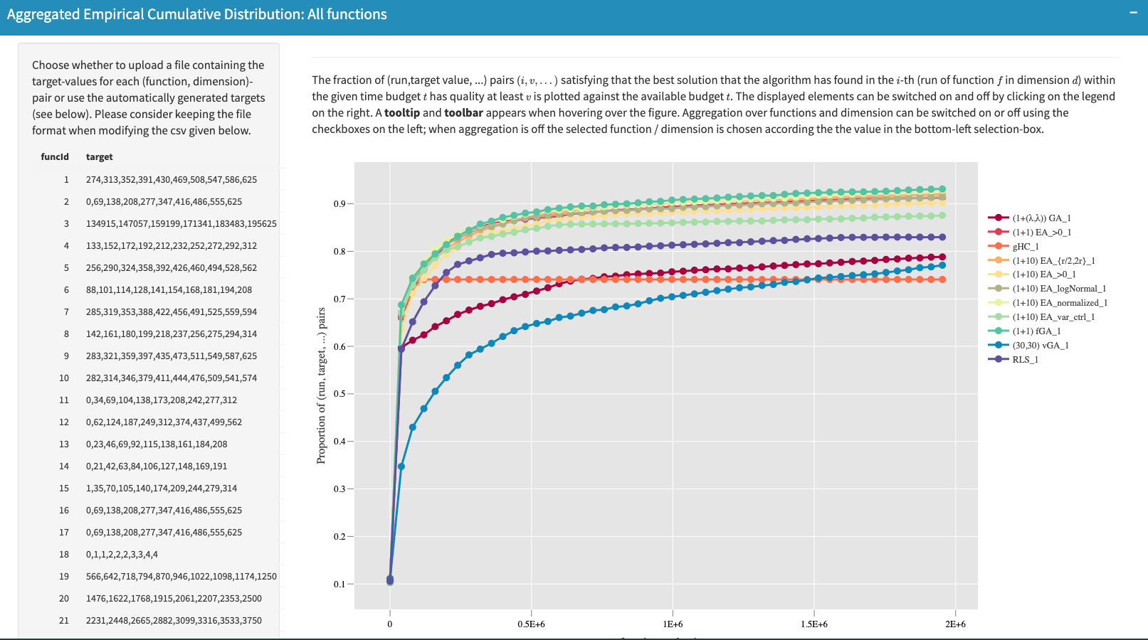
In the example figure, a table of pre-calculated target values are provided for each test function while all 23 test functions are considered here by default. This table could also be customized by

1. Downloading the current table (in a CSV-like format)
2. Modifying it according to user’s preference
3. Uploading the modified table again.

The plot on the right will be re-computed upon uploading a new table of targets. Note that the format of the example table should be retained while editing it to make sure it can be read when uploaded.