Algorithms

As a demonstration of the proposed benchmarking environment, some basic experimental results have been reported in the paper Benchmarking discrete optimization heuristics with IOHprofiler. The implementation of algorithms can be found in the repository IOHalgorithm.

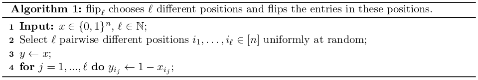
A detailed description of the algorithms follows. An operator frequently used in these descriptions is the \(flip(\cdot)\) mutation operator, which flips the entries of \(\ell\) pairwise different, uniformly at random chosen bit positions, see Algorithm 1.

Since we want to avoid useless evaluations of offspring that are identical to their parents, we frequently make use of the conditional binomial distribution \(Bin_{>0}(n,p)\), which assigns probability \(Bin(n,p)(k)/(1-(1-p)^n)\) to each positive integer \(k \in [n]\), and probability zero to all other values. Sampling from \(Bin_{>0}(n,p)\) is identical to sampling from \(Bin(n,p)\) until a positive value is returned (“resampling strateg”).

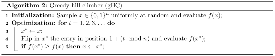
Greedy Hill Climber

The greedy hill climber (gHC, Algorithm 2) uses a deterministic mutation strength, and flips one bit in each iteration, going through the bit string from left to right, until being stuck in a local optimum, see Algorithm 2.

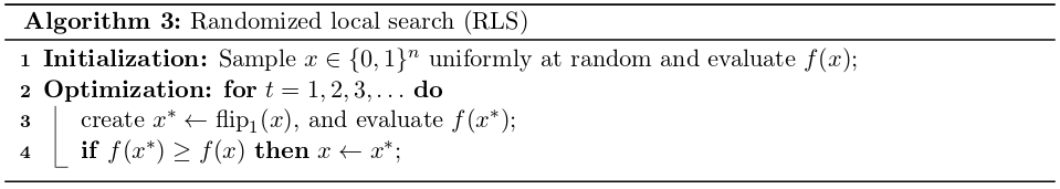
Randomized Local Search

RLS uses a deterministic mutation strength, and flips one randomly chosen bit in each iteration, see Algorithm 3.

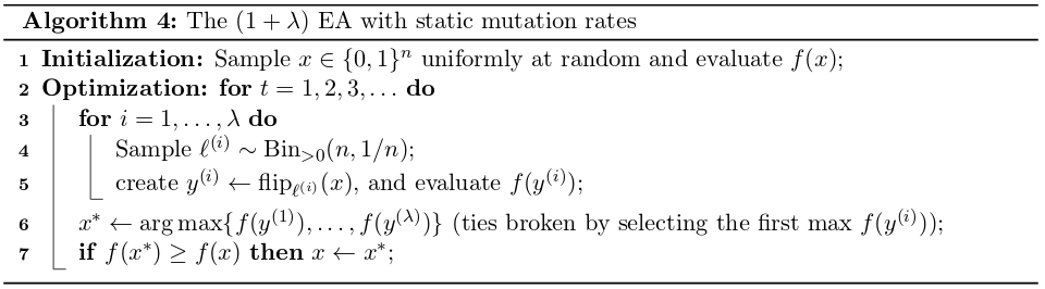
The EA with Static Mutation Rate

The \((1+\lambda)\) EA is defined via the pseudo-code in Algorithm 4.

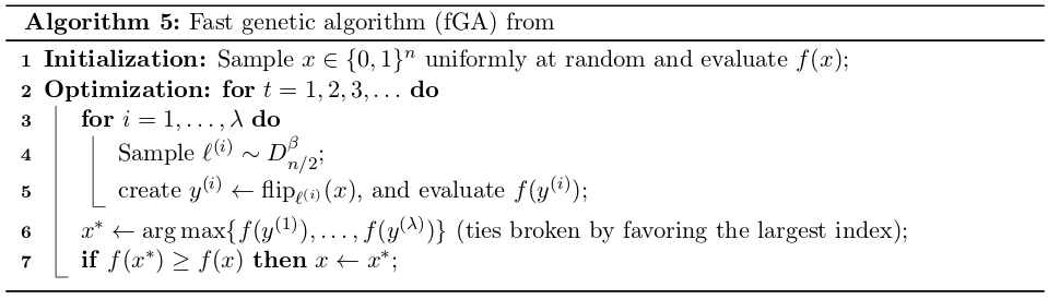
Fast Genetic Algorithm

The fast Genetic Algorithm (fGA) chooses the mutation length \(\ell\) according to a power-law distribution \(D^\beta_{n/2}\), which assigns to each integer \(k \in [n/2]\) a probability of \(Pr[D^\beta_{n/2}] = (C^\beta_{n/2})^{-1}k^{-\beta}\), where \(C^\beta_{n/2} = \sum^{n/2}_{i=1}i^{-\beta}\). We use this algorithm with \(\beta = 1.5\). The fGA was introduced in the paper Fast genetic algorithms.

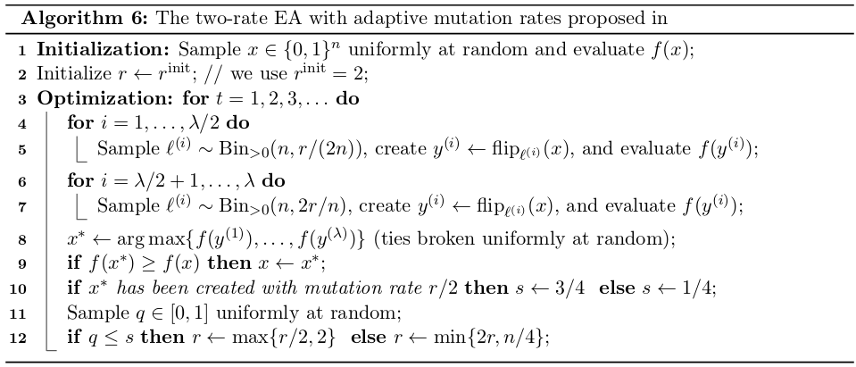
The Two-Rate EA

The two-rate \((1+\lambda) EA_{r/2,2r}\) was introduced in the paper The \((1+\lambda)\) Evolutionary Algorithm with Self-Adjusting Mutation Rate. It uses two mutation rates in each iteration: half of offspring are generated with mutation rate \(r/2n\), and the other \(\lambda/2\) offspring are sampled with mutation rate \(2r/n\). The parameter \(r\) is updated after each iteration, from a biased random decision favoring the value from which the best of all \(\lambda\) offspring has been sampled.

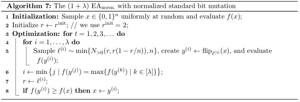
The EA with normalized standard bit mutation

The \((1+\lambda) EA_{norm.}\), Algorithm 7, samples the mutation strength from a normal distribution with mean \(r = pn\) and variance \(pn(1-p) = r(1-r/n)\), which is identical to the variance of the binomial distribution used in standard bit mutation. The parameter \(r\) is updated after each iteration, in a similar fashion as in the 2-rate EA, Algorithm 6. The \((1+\lambda) EA_{norm.}\) was introduced in the paper Interpolating Local and Global Search by Controlling the Variance of Standard Bit Mutation.

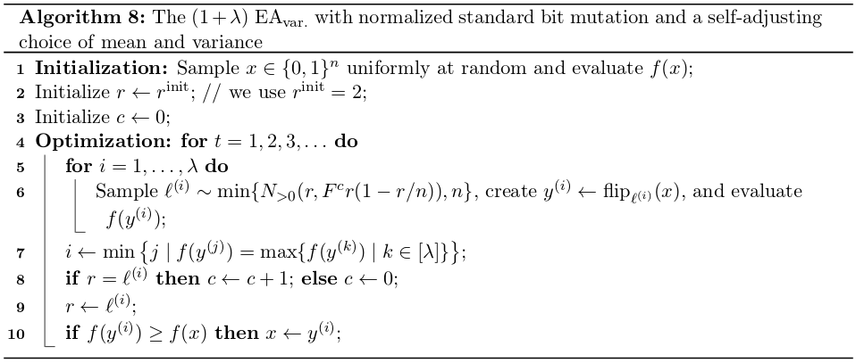
The EA with normalized standard bit mutation and controlled variance

The \((1+\lambda) EA_{var.}\), Algorithm 8 builds on the \((1+\lambda) EA_{norm.}\) but uses, in addition to the adaptive choice of the mutation rate, an adaptive choice of the variance.

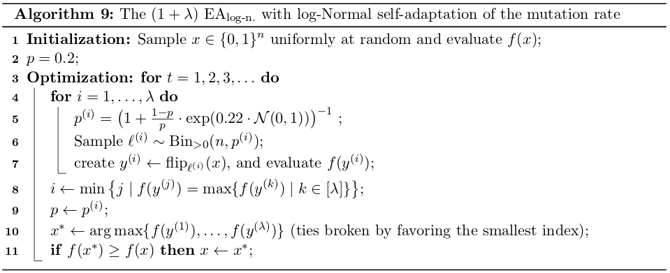
The EA with log-Normal self-adaptation on mutation rate

The \((1+\lambda) EA_{log-n}\), Algorithm 9, uses a self-adaptive choice of the mutation rate.

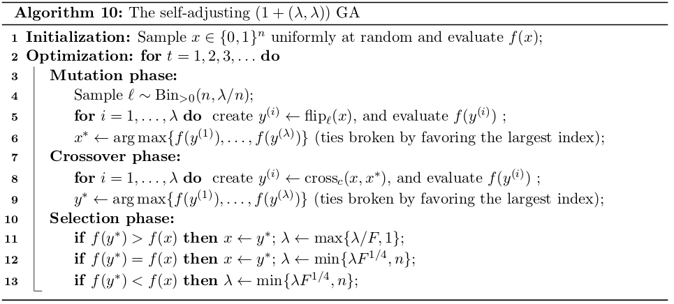
The Self-Adjusting \((1+(\lambda+\lambda)) GA\)

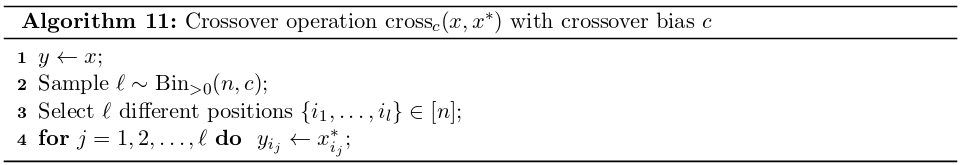
The self-adjusting \((1+(\lambda+\lambda)) GA\), Algorithm 10, was introduced in the paper From black-box complexity to designing new genetic algorithms. The offspring population size \(\lambda\) is updated after each iteration, depending on whether or not an improving offspring could be generated. Since both the mutation rate and the crossover bias (see Algorithm 11 for the definition of the biased crossover operator cross) depend on \(\lambda\), these two parameters also change during the run of the \((1+(\lambda+\lambda)) GA\). In our implementation we use update strenght \(F=3/2\).

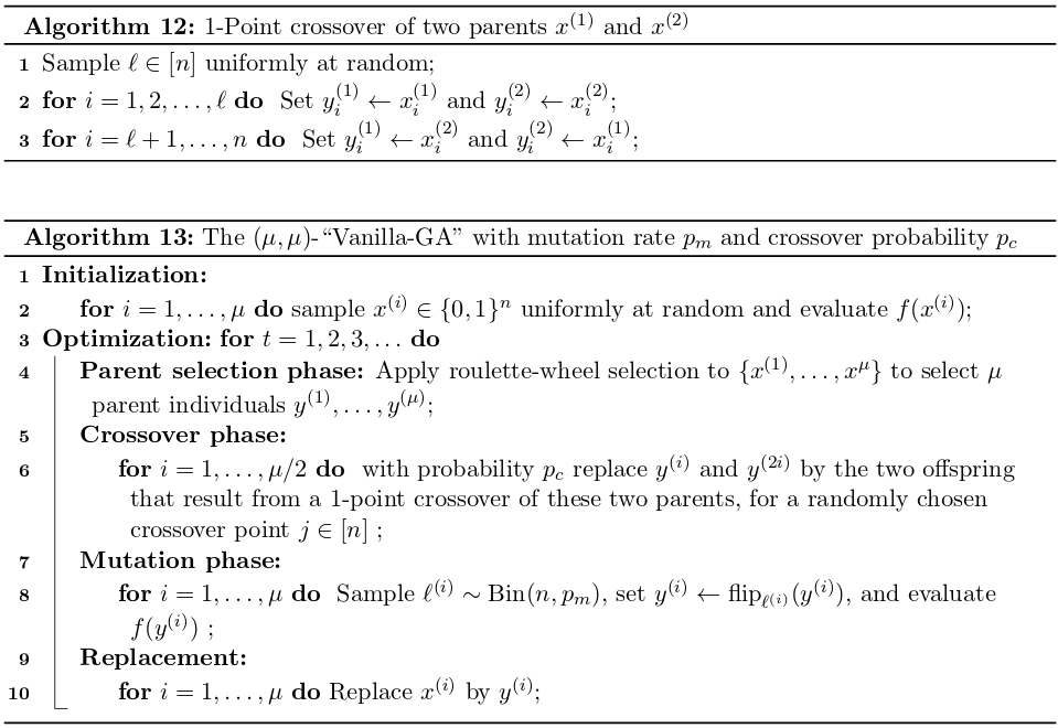
The “Vanilla” GA

The vanilla GA (vGA, Algorithm 13) constitutes a textbook realization of the so-called Traditional GA. The algorithm holds a parental population of size \(\mu\). It employs the Roulette-Wheel-Selection (RWS, that is, probabilistic fitness-proportionate selection which permits an individual to appear multiple times) as the sexual selection operator to form \(\mu/2\) pairs of individuals that generate the offspring population. 1-point crossover (Algorithm 12) is applied to every pair with a fixed probability of \(p_c = 0.37\). A mutation operator is then applied to every individual, flipping every bit with a fixed probability of \(p_m = 2/n\). This completes a single cycle.

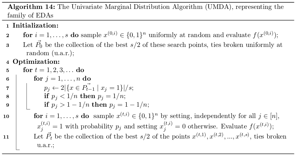
The Univariate Marginal Distribution Algorithm

The univariate marginal distribution algorithm (UMDA, Algorithm 14) is one of the simplest representatives of the family of so-called estimation of distribution algorithms (EDAs). The algorithm maintains a population of size \(s\) and uses the best \(s/\) of these to estimate the marginal distribution of each decision variable, by simply counting the relative frequency of ones in the corresponding position. These frequencies are capped at \(1/n\) and \(1-1/n\), respectively. In the \(t\)-th iteration, a new population is created by sampling from these marginal distributions. The UMDA was introduced in The Equation for Response to Selection and Its Use for Prediction.